
Students will explore a predator-prey relationship in the ocean using the VES-V software. Students will compare the population trends of a predator (cod) and one of its prey (mackerel). Students will observe the trend over time of cod biomass in the Gulf of Maine. Based on the trend in cod biomass, students will predict the trend in mackerel (prey) biomass. Students will then look at the graph of mackerel biomass in VES-V to test their hypothesis. Students will follow these steps twice, first using data generated by a model, then using data from observations.
NOTE: Biomass Review - Data about fish populations in VES-V are provided in terms of total biomass of a given species, not in terms of the population count of individual organisms. Since the examples used earlier in this lesson, with lynx and hares, were expressed in terms of the population of individuals, you may want to review the concept of biomass to make sure students are clear about the distinction. Also, if biomass is a new or relatively unfamiliar concept for your students, you might want to discuss biomass before students “dive” into VES-V.
Biomass is the total amount of mass of living creatures of a given type or in a certain area. For example, one could describe the total biomass of fish in a cubic kilometer of ocean, or the biomass of all jellyfish. Biomass is the total number of organisms multiplied by the mass of each creature. If the average mass is known, multiplying that mass by the population count gives the biomass. A single, large adult fish contributes more to biomass than a small, juvenile fish does. However, there may be many, many more smaller fish than larger ones, so the many small fish might contribute more to total biomass than a few larger fish do. A large school of sardines might outweigh a single whale.
A simple thought experiment might help your students with the concept of biomass. An average 1st-grader weighs around 45 pounds (about 20 kg). A class of 25 1st grade students would have a biomass of around 1,125 pounds ( = 45 x 25) or 500 kg. A typical high school senior weighs around 130 pounds (nearly 60 kg). A class of 20 high school seniors, 5 fewer than the first grade class, would have a biomass around 2,600 pounds ( = 130 x 20) or 1,200 kg. Even though there are fewer high school seniors than 1st graders in this example, the biomass of the high school students is more than twice as large as the biomass of elementary students.
Students will collect data about a predator, cod, within the VES-V software. Ask students to conduct a virtual dive in the Northeast region in the Gulf of Maine and select the sand flats habitat. The dataset for the “Baseline” scenario loads by default. Have students load a different dataset by clicking the green “SCN” (scenario) folder icon in the upper left and switch to the NEFSCassessment scenario. Inform students that this dataset is based on a model.
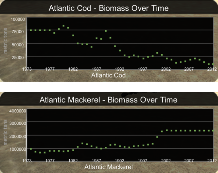
Ask students to click on the Atlantic Cod icon along the left edge of the screen. The biomass graph (Figure 8) shows cod biomass from 1973 to 2012. Ask students to identify the overall trend of cod biomass across this graph. Is it increasing, decreasing, or staying about the same? Students should easily see that the overall trend is decreasing biomass.
Next, ask students to predict the biomass trend for a type of fish that cod eat. Do students think that the biomass of the prey species will increase, decrease, or stay about the same in response to the decline in predator (cod) biomass?
Students will now test their hypothesis. Have students click on the icon for Atlantic Mackerel to display a graph of mackerel biomass (Figure 8) and ask them to describe the overall trend in mackerel biomass. Is it increasing, decreasing, or staying the same? Students should observe that mackerel biomass generally increases between 1973 and 2012.
Ask students to compare their prediction about the trend in mackerel biomass with the data they just observed. Was their hypothesis correct? Does the relationship between cod and mackerel biomass follow the basic patterns that students observed earlier in the lynx and hare predator-prey system?

Figure 8: Cod and Mackerel Biomass from the NEFSCassessment Dataset
Have students switch to a different dataset. Using the sand flats habitat in the Gulf of Maine select the NEFSCsurveytrawlandMammalBird dataset by clicking on the green “SCN” (scenario) folder icon in the upper left. Inform students that this dataset is based on observations, as compared to the previous dataset they used which was based on a model.
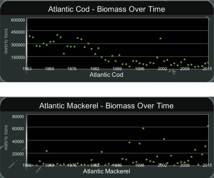
Once again, have students observe the biomass graph for cod by clicking the cod icon along the edge of the screen. Figure 9 shows the biomass for cod from 1963 to 2015.
Ask students to once again identify the trend in the data. Was cod biomass generally increasing, decreasing, or staying the same over the course of the graph? It should be apparent that the overall trend in cod biomass was decreasing.
As with the model data, ask students to predict the trend in prey (mackerel) biomass in response to this decrease in predator (cod) biomass.
Have students observe the mackerel biomass graph (which is shown in Figure 9). Although this graph is “messy” and more erratic than the previous examples, there are far more high values of mackerel biomass toward the right side of the graph. Overall, the mackerel biomass does seem to be increasing.
Ask students to compare their hypothesis about the trend in mackerel biomass with the actual mackerel data. Also ask students whether these results make sense to them. What would they expect to happen to a prey species like mackerel when there are fewer predators around?
Have students record their observations and predictions about cod and mackerel biomass trends in the tables on “VES-V Predator-Prey Lesson Worksheet #2: Cod and Mackerel Biomass Trends”.

Figure 9: Cod and Mackerel Biomass from the NEFSCsurveytrawlandMammalBird Dataset
NOTE: Biomass Review - Wrap up this activity by making some comparisons. Remind students that real-world, observational data is often messy and more erratic than the smoother trends predicted by models. This is evident in both the cod and mackerel data from VES-V and in the lynx and hare data from the spreadsheet model and the historical Hudson Bay Company record.
The cod and mackerel data from VES-V does not show the repeating cycles of rising and falling populations that are evident in the lynx and hare model and historical data.
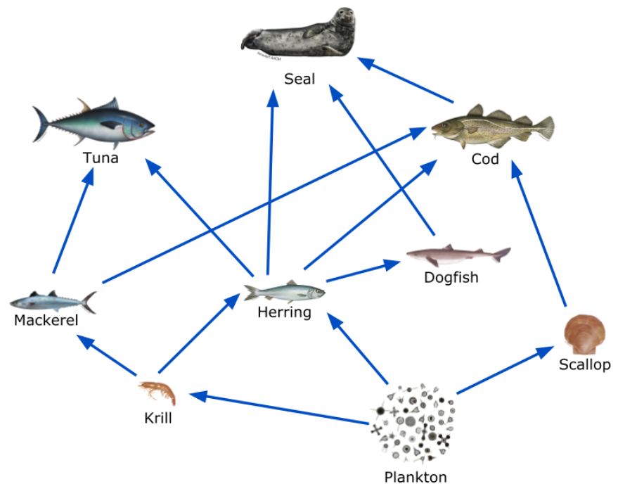
Cod and mackerel are part of a complex food web, part of which is shown in Figure 10. This is a much different situation from the simple single predator and single prey system modeled in the spreadsheet.
We should not expect such a simple pattern of repeatedly rising and falling populations to arise in a complex food web or marine system due to the multitude of biotic and abiotic factors affecting the many species in the food web.
The cod and mackerel data may show part of one of those repeating cycles akin to the lynx and the hare if data from observations were carried out over very long periods of time.

Figure 10: Partial Food Web Including Cod and Mackerel