[ Modeling Marine Ecosystems with Virtual Reality: NOAA's National Ocean Service

U.S. flag An official website of the United States government.

dot gov icon Official websites use .gov

A .gov website belongs to an official government organization in the United States.

https icon Secure websites use HTTPS

A small lock or https:// means you’ve safely connected to a .gov website. Share sensitive information only on official, secure websites.

Predators and prey

Predators and Prey Module

Activity II: Setting up a Predator-Prey Model

Activity Summary

Students will discuss the factors that define a predator-prey model and investigate a simple relationship between a single predator and a single prey species. Throughout this activity students learn how birth rate, death rate, and rate of predation control the behavior of this simple population model. Students will also set up a simple predator-prey model in a spreadsheet program, run this model and analyze the results from it in the upcoming activities in this lesson.

Procedure:

NOTE: As a teacher, you have three options for this activity. The first option takes the least time and does not require your students to have computer expertise. Options two and three require more time and involve progressively more computer expertise. Options two and three also provide a more in-depth look “under the hood” of the process of constructing a model.

Option One: Discuss with students the factors and considerations that go into making a predator-prey model. Do not construct or manipulate a model. Then skip ahead to “Activity IV: Analyzing Results of a Predator-Prey Model”, which involves analysis of a graph of results from the model.

Option Two: Demonstrate the model spreadsheet to students as a whole-class activity. You can either construct the model in a spreadsheet from scratch, or you can use a preconfigured version.

Option Three: Have students interact with the spreadsheet model directly, either after constructing the model themselves or with a copy of a preconfigured version of the model in a spreadsheet.

Option 3 requires a higher level of student expertise with computers in general and spreadsheet software in particular. The first part of this activity (below) describes a discussion with students about the elements of a predator-prey model. You should conduct that discussion in each of the three options described above. The rest of the description of this activity assumes that you are using option 3 and having students construct the model in a spreadsheet. If you choose to follow the option 1 or 2 approach instead, adjust your lesson accordingly.

If you don’t want to construct the spreadsheet version of the model yourself, and you don’t want students to build the model, this zipped file provides a comma-separated values (CSV) document, which you can import into an Excel spreadsheet or a Google Sheet. The zipped file also contains an image depicting an example of the model that you can construct from this data.

  1. Discussion: Ask your students to imagine an area that is home to lots of rabbits. If there was enough food for the rabbits in that area, the rabbits would have lots of babies and the rabbit population would grow. Now imagine that some sort of predator, such as foxes or wolves or coyotes, moved into the rabbits’ range. The predators would find lots of food (rabbits), and would in turn have baby predators. The predator population would grow, but the rabbit population might shrink. What would happen to the rabbit and predator populations over time? Mention to students that scientists use mathematical models to predict the future status of systems like the predator-prey example just described. In this activity, we will consider the factors that should be included in a very simple predator-prey model. Students will incorporate those factors into a model using spreadsheet software. In the next activity, students will run the model to see what it predicts.

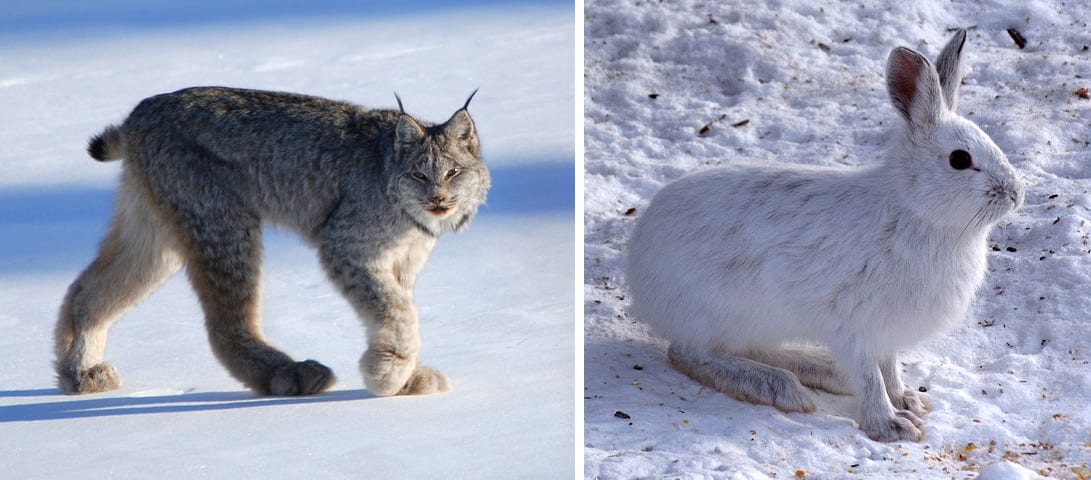
    a Canadian Lynx and a snowshoe hare

    Figure 1: Canadian Lynx and Snowshoe Hare

    NOTE: Later in this module, during Activity V, students will look at historical data about a specific predator and its prey.

  2. Via lecture/short presentation introduce students to a predator prey relationship. The predator in that case study is the Canada lynx, a type of medium-sized wild cat found throughout Canada and Alaska. The prey species in the historical case study is the snowshoe hare, a type of rabbit that is also widespread throughout Canada and Alaska.

  3. Construct the predator-prey model.
    • To begin constructing the predator-prey model, ask students to think about the factors that influence the size of the snowshoe hare population and develop a mathematical representation of that relationship. For example: some new hares are born, increasing the population. Some hares die, decreasing the population. A simple equation representing the change in hare population looks like:

      Change in Hare Population = Hare Births - Hare Deaths

      NOTE: In this simple model, we will assume the hares always have access to enough food. The number of hare births will only depend on the number of hares. For example, if one new hare is born each month for every ten hares in the population, we would expect a population of 500 hares to produce about 50 babies each month, or a population of 2,000 hares to produce 200 offspring.

      Similarly, we would expect the number of hares that die due to old age or illness to also depend on the number of hares. There would be many more deaths in a population of 2,000 hares than in a population of 200 hares, but the fraction of the population that dies is expected to be about the same. However, the hares are preyed upon by the lynx, and don’t just die of old age or illness. Most hare deaths are caused by predation by lynx. Therefore, there would be more hare deaths when there are lots of lynx, and fewer hare deaths if the lynx population was low. So, unlike the hare birth rate which is only influenced by the size of the hare population, the hare death rate depends on both the size of the hare population and the size of the lynx population.

    • Ask students to hypothesize when the hare population might grow, and when it might shrink. For example, if the birth rate is greater than the mortality rate, the hare population would increase.

      NOTE: The mortality rate for hares depends on how many lynx there are eating hares. If there are few lynx, few hares get eaten, the hare birth rate is larger than the hare death rate, and the hare population would be expected to increase. On the other hand, if there are lots of lynx, many hares would get eaten, hare deaths would outpace births, and the hare population would likely decline. In short, when there are few lynx, the hare population would grow; when there are many lynx, the hare population would shrink.

    • Ask students to revise their Change in Hare Population equation to reflect the predator prey relationship.
    • Next, invite students to consider factors that influence the size of the lynx population. As is the case with hares, the change in the lynx population can be modeled with a simple equation:

      Change in Lynx Population = Lynx Births - Lynx Deaths

      NOTE: In this case, since there aren’t any predators killing lynx, the number of lynx deaths should only depend on the number of lynx. If 1 out of 100 lynx die in a month, we would expect 20 deaths if the lynx population was 2,000, and so on. The number of lynx deaths follows the same pattern as hare births; it only depends on the population size. On the other hand, the number of lynx births depends on the food supply.

      Lynx produce more offspring when food is plentiful, and have fewer kittens when less food is available. Since Snowshoe Hares are the main food source for lynx, the availability of hares as food plays a major role in lynx population change. Like hare deaths, the rate of lynx births depends on both the lynx population size and on the hare population size. When there are many hares for lynx to eat, lynx births increase and so does the lynx population size. When there are fewer hares for lynx to eat, fewer lynx are born and the lynx population decreases.

  4. Set up and run the Hare-Lynx Model in a spreadsheet. Inform students that the next step is to translate these ideas into equations in a spreadsheet. The spreadsheet model will have a time step size of one month; it will assume one month of time has passed every time the new values for lynx population and hare population are calculated.

    The equations to calculate the new value for the hare population are:

    Number of Hare Births = k1 x (# of Hares)
    Number of Hare Deaths = k2 x (# of Hares) x (# of Lynx)
    Change in Hare Population = (# of Hare Births) - (# of Hare Deaths)
    New Hare Population = Previous Hare Population + Change in Hare Population

    NOTE: The values k1 and k2 are constants. If k1 equals 0.01, then there would be one hare birth each month for every 100 hares. Similarly, k2 adjusts the total number of hare deaths. As previously discussed, the number of births depends on just the number of hares, while the number of deaths depends on both the number of hares and of lynx.

    The equations to calculate lynx populations in the spreadsheet are similar, reusing the constant k2 and introducing a third constant, k3, which controls lynx mortality rate.

    Number of Lynx Births = k2 x (# of Hares) x (# of Lynx)
    Number of Lynx Deaths = k3 x (# of Lynx)
    Change in Lynx Population = (# of Lynx Births) - (# of Lynx Deaths)
    New Lynx Population = Previous Lynx Population + Change in Lynx Population

    NOTE: The number of lynx births depends on both the number of hares (food availability) and the number of lynxes (prospective parents). The number of lynx deaths is proportional to the number of lynx, since in this simple model we assume there are no predators of lynx so lynx deaths result only from “natural” causes such as disease or old age.

Guidance: Creating the Model in a spreadsheet

  1. Open up your spreadsheet program and create a new blank sheet.
  2. Copy the values and formulas from the table below into the spreadsheet.
  3. You can see how this model is constructed in this sample spreadsheet.

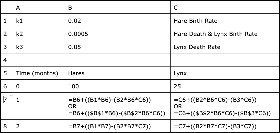
Table 1 (below) shows the values to enter into a spreadsheet program to set up this predator-prey simulation model.

  • This table illustrates the first 8 rows and 3 columns (A, B and C) of cells in a spreadsheet.
  • These values can be used with any of the common spreadsheet programs, such as Microsoft Excel, Google Sheets, or Apple Numbers.
  • The values for the constants (k1, k2 and k3) are in rows 1-3 of column B.
  • Time in the simulation, in months, appears in column A, starting with time zero in row 6.
  • Columns B and C of row 6 list the initial values for the hare and lynx populations. These initial values are arbitrary.
  • Row 7 contains the first calculations of future populations in the model, in columns B and C.
  • Cell B7 contains the new hare population, calculated using the equations described above. The calculation in cell B7 includes the previous hare population (B6 = 100), the number of hare births (B1*B6), and the number of hare deaths (B2*B6*C6).
  • Similarly, cell C7 contains the calculation for the lynx population after one month.
  • Predator-Prey Model Setup in a Spreadsheet

    Table 1: Predator-Prey Model Setup in a Spreadsheet

  • Row 8 of Table 1 repeats the hare and lynx population calculations, this time using the population values from the first month (row 7) as the starting point.
  • We recommend that this spreadsheet model include about 600 months of data. Once the formulas have all been entered correctly, highlight the bottom three columns and click and drag the resulting box down the sheet to the desired number of rows (600). If desired, you can practice this method on the provided spreadsheet.
  • Rows 7 and 8 in Table 1 show the pattern for the first two months, which should be repeated in further spreadsheet rows for the remaining 598 months.

Spreadsheet Insights: If you and your students are familiar with the special notations that are used in spreadsheets, students should note that the “$” notation is used when referring to the values of the constants k1, k2 and k3 in cells B1, B2 and B3. The “$” notation makes fixed, as opposed to relative, reference to a specific cell in a spreadsheet, making it easier to autofill a formula into a series of cells. In Table 1, the cell references “B1”, “B2” and “B3” in the formulas starting in row 7 are changed to “$B$1”, “$B$2” and “$B$3”. Use of this notation makes it simpler to autofill formulas and values for hare and lynx populations into spreadsheet rows representing month 2 and beyond.

NOTE: If students set up the spreadsheet correctly, the hare population in month 1 (spreadsheet row 7) should be 100.75, a slight increase from the initial value of 100. Students may ask what it means to have an extra 0.75 hare. Obviously there are no partial hares. In the real world, there might be 1 new hare, or there might be 0 new hares. Remind students that this is a model, and models are not the same as the real world in every way. One way to think of the 0.75 hare could be that there is about a 75% chance that the hare population would increase by 1 hare during the first month (and a 25% chance that there would be no increase).

The lynx population in month 1 stays the same as the starting value for lynx of 25. It just happens that the number of lynx deaths is exactly the same as the number of lynx births during the first month, so the lynx population does not change from the start to month 1. By month 2 the lynx population slowly starts to climb, inching upward to about 25.01 lynx. The population slowly creeps upward from there, reaching 26 lynx by the 15th month. As with the hare population, the model produces fractional lynx populations which don’t mean there are parts of lynx running around.